Visualizing 3D Leg Muscle Anatomy from STL Files

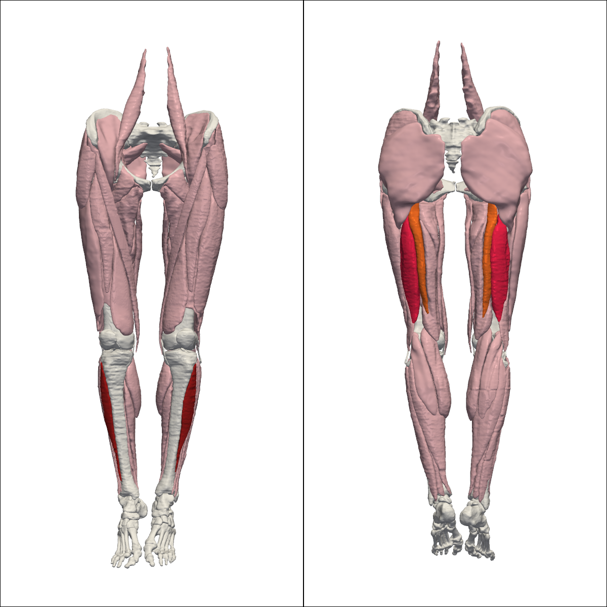
We created 12 realistic muscle geometries based on segmentations of the Visible Human dataset (Andreassen et al., 2023). These include the tibialis anterior, biceps femoris long head, and semitendinosus muscles for both left and right legs, male and female.

In this script, we use PyVista to visualize these 3D muscle geometries with custom coloring for different tissue types and specific muscles.

import pyvista as pv
from pathlib import Path

pv.set_jupyter_backend("static")
surfaces_path = Path("..") / "data" / "VHF_surfaces"

The tibialis anterior is shown in dark red, the biceps femoris long head in bright red, and the semitendinosus in orange. Non-highlighted muscles are soft pink, whereas bones and other tissues are white.

color_ta = "#B22020"  # dark red
color_bflh = "#FF2752"  # bright red
color_st = "#FF7429"  # orange

custom_highlights = {
    "VHF_Left_Muscle_TibialisAnterior_smooth.stl": color_ta,
    "VHF_Right_Muscle_TibialisAnterior_smooth.stl": color_ta,
    "VHF_Left_Muscle_BicepsFemorisLong_smooth.stl": color_bflh,
    "VHF_Right_Muscle_BicepsFemorisLongHead_smooth.stl": color_bflh,
    "VHF_Left_Muscle_Semitendinosus_smooth.stl": color_st,
    "VHF_Right_Muscle_Semitendonosus_smooth.stl": color_st,
}

tissue_colors = {
    "Bone": "#FFFFFF",
    "Muscle": "#F8C4CF",
    "Ligament": "#FFFFFF",
    "Cartilage": "#FFFFFF",
}

We now load all STL files from the specified directory and visualize them with PyVista.

plotter = pv.Plotter(shape=(1, 2), window_size=[1200, 1200], off_screen=True)
plotter.set_background("white")


loaded_count = 0

for filepath in surfaces_path.rglob("*.stl"):
    filename = filepath.name

    # --- Logic to determine color/style ---
    if filename in custom_highlights:
        color = custom_highlights[filename]
        specular = 0.5
    elif "_Bone_" in filename:
        color = tissue_colors["Bone"]
        specular = 0.1
    elif "_Muscle_" in filename:
        color = tissue_colors["Muscle"]
        specular = 0.2
    elif "_Ligament_" in filename:
        color = tissue_colors["Ligament"]
        specular = 0.3
    elif "_Cartilage_" in filename:
        color = tissue_colors["Cartilage"]
        specular = 0.4

    mesh = pv.read(filepath)

    # Add to both subplots
    plotter.subplot(0, 0)
    plotter.add_mesh(mesh, color=color, specular=specular)
    plotter.subplot(0, 1)
    plotter.add_mesh(mesh, color=color, specular=specular)

    loaded_count += 1

print(f"Total parts loaded from {surfaces_path}: {loaded_count}")

# Front View
plotter.subplot(0, 0)
plotter.view_xz(negative=True)
plotter.camera.zoom(1.8)

# Back View
plotter.subplot(0, 1)
plotter.view_xz(negative=False)
plotter.camera.zoom(1.8)

# Render the combined image
plotter.show()

2026-01-09 15:15:58.047 (   0.561s) [    7F1E5EFAF140]vtkXOpenGLRenderWindow.:1458  WARN| bad X server connection. DISPLAY=:99.0

Total parts loaded from ../data/VHF_surfaces: 128

output_file = Path("..") / "results" / "geometries" / "anatomy_view.png"
output_file.parent.mkdir(parents=True, exist_ok=True)
plotter.screenshot(output_file, scale=4)
print(f"Anatomy view saved to: {output_file}")

Anatomy view saved to: ../results/geometries/anatomy_view.png