Simulation of the IGF1-AKT-mTOR-FOXO Pathway

This demo illustrates the use of the IGF1-AKT-mTOR-FOXO signaling model to simulate muscle adaptation.

The model represents a key biochemical pathway regulating muscle hypertrophy:

1. Exercise Stimulus: Exercise triggers the release of IGF1 and activation of AKT.

2. Protein Balance: AKT promotes protein synthesis via mTOR and inhibits protein degradation by suppressing FOXO.

3. Outcome: The net balance determines the change in the myofibril population (N).

We will define an exercise protocol and visualize how these molecules respond over time.

from musclex.exercise_model import ExerciseModel
from musclex.protocol import RegularExercise
from matplotlib import pyplot as plt
import matplotlib.gridspec as gridspec
from pathlib import Path

config = Path("../config_files/exercise_eq_reduced_k1.yml")
results = Path("../results/demos/signaling_demo")
results.mkdir(parents=True, exist_ok=True)

Define the exercise protocol

An exercise protocol is defined by the frequency, duration, and intensity of exercise sessions. This protocol consists of 7 exercise sessions, each lasting 1 hour, with 47 hours of rest between sessions. The total duration is 15 days, and each session is performed at 80% of maximum intensity.

protocol = RegularExercise(
    N=7, exercise_duration=1, growth_duration=47, end_time=15 * 24, intensity=0.8
)

# Print protocol details
fmt = lambda t: f"Day {int(t//24)}, {t%24:04.1f}h"
print(f"{'TYPE':<15} {'START':<15} {'END':<15} {'DURATION'}")
for e in protocol.events:
    print(
        f"{type(e).__name__:<15} {fmt(e.start_time):<15} {fmt(e.end_time):<15} {e.end_time-e.start_time:.1f}h"
    )

TYPE            START           END             DURATION
ExerciseEvent   Day 0, 00.0h    Day 0, 01.0h    1.0h
GrowthEvent     Day 0, 01.0h    Day 2, 00.0h    47.0h
ExerciseEvent   Day 2, 00.0h    Day 2, 01.0h    1.0h
GrowthEvent     Day 2, 01.0h    Day 4, 00.0h    47.0h
ExerciseEvent   Day 4, 00.0h    Day 4, 01.0h    1.0h
GrowthEvent     Day 4, 01.0h    Day 6, 00.0h    47.0h
ExerciseEvent   Day 6, 00.0h    Day 6, 01.0h    1.0h
GrowthEvent     Day 6, 01.0h    Day 8, 00.0h    47.0h
ExerciseEvent   Day 8, 00.0h    Day 8, 01.0h    1.0h
GrowthEvent     Day 8, 01.0h    Day 10, 00.0h   47.0h
ExerciseEvent   Day 10, 00.0h   Day 10, 01.0h   1.0h
GrowthEvent     Day 10, 01.0h   Day 12, 00.0h   47.0h
ExerciseEvent   Day 12, 00.0h   Day 12, 01.0h   1.0h
GrowthEvent     Day 12, 01.0h   Day 15, 00.0h   71.0h

Initialize and run the model

The simulate method runs the simulation event by event based on the defined exercise protocol.

model = ExerciseModel(protocol, str(config), results)
model.simulate()

Visualize the results

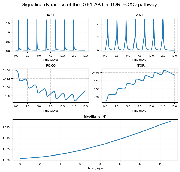
We plot the time courses of IGF1, AKT, FOXO, mTOR, and the myofibril population (N) over the simulation period.

state_names = ["IGF1", "AKT", "FOXO", "mTOR", "Myofibrils (N)"]
t_days = model.t / 24

fig = plt.figure(figsize=(7, 7))
gs = gridspec.GridSpec(3, 2, height_ratios=[1, 1, 1.2])
axes = [
    plt.subplot(gs[0, 0]),  # IGF1
    plt.subplot(gs[0, 1]),  # AKT
    plt.subplot(gs[1, 0]),  # FOXO
    plt.subplot(gs[1, 1]),  # mTOR
    plt.subplot(gs[2, :]),  # Myofibrils
]
for i, ax in enumerate(axes):
    ax.plot(t_days, model.y[i, :], color="#1f77b4", linewidth=2)
    ax.set_title(state_names[i], fontweight="bold")
    ax.grid(True, linestyle="--", alpha=0.6)
    ax.set_xlabel("Time (days)")
plt.suptitle("Signaling dynamics of the IGF1-AKT-mTOR-FOXO pathway", fontsize=14, y=0.96)
plt.tight_layout(rect=[0, 0.03, 1, 0.96])
plt.show()